Tutorial: Assessing coupling dynamics
In this tutorial we will characterize temporal coupling dynamics between several scalar time-series using the function transfer_entropy_pt.m, which is included in TIM Matlab interface.
Tutorial files
Here are the Matlab scripts that are used in this tutorial.
We have implemented all the tutorial steps in just three Matlab functions: tutorial_gauss_data.m, tutorial_gauss_analysis.m, and tutorial_gauss_figures.m. These functions generate the data, perform the connectivity analysis, and generate the figures, respectively. You can obviously reproduce the final results of the tutorial by simply running those three files. However, the purpose of this tutorial is to teach you how to perform the connectivity analysis yourself. That is why we will ignore function tutorial_gauss_analysis.m until the end of this tutorial.
Problem statement
We consider the following non-linearly coupled Gaussian processes with a time-varying coupling factor:
where the index corresponds to the trial (or repetition) index and denotes time instants. The terms , and are normally distributed noise processes, which are mutually independent across trials and time instants. The coupling delays are fixed to , and the coupling strength is modulated using the following time-varying coupling factors:
The problem is to reveal the temporal coupling between the time series x, y, and z.
Data generation
The following function generates these time-series:
data = tutorial_gauss_data();
This loads a cell-array data of dimensions 3 x 50. The rows of this
cell array correspond to the x, y, and z time-series and the columns
contain different random repetitions.
Results
We will begin by showing what results to except from the analysis. We have implemented the whole analysis in function tutorial_gauss_analysis.m so, if you are feeling lazy, simply run:
tutorial_gauss_analysis;
This command will save the whole analysis results into a file called
tutorial_gauss_analysis.mat. Then, to generate some nice figures you can
run:
tutorial_gauss_figures;
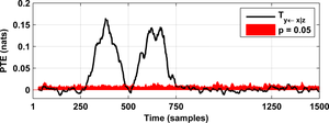
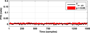
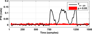
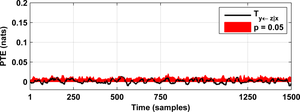
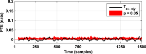
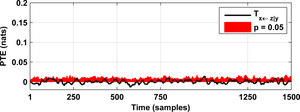
As a result you will obtain the following figures:
State-space reconstruction
Let us assume that we have measured , and and that we want to infer the underlying connectivity pattern and the corresponding coupling dynamics. Before anything else, we have to reconstruct the state-space of these scalar time-series, which can be done using delay embedding (motivated by the Taken’s delay embedding theorem):
dim = 1, tau = 1;
Sx = delay_embed(data(1, :), dim, tau);
Sy = delay_embed(data(2, :), dim, tau);
Sz = delay_embed(data(3, :), dim, tau);
where dim and tau are the embedding dimension and the embedding delay,
respectively. Choosing the right embedding parameters can be a tricky
issue. The simplest way is to take tau = 1 and successively embed in
higher dimensions until the results of the analysis are consistent.
However, there are several more advanced techniques
that you may want to try. For a comprehensive review on delay embedding
and state-space reconstruction, we recommend you this book
by Holger Kantz and Thomas Shreiber, two well-known
experts in the field. In our case, the default choice of tau = 1 and
dim = 1 will produce satisfactory results, as we will see later.
Of course, this embedding does not change the data in any way.
However, that no higher-dimensional embedding is needed is specific for
this tutorial problem, and does not hold for problems in general. Choosing
a right delay-embedding is necessary for a successful analysis;
that is why we have included it here explicitly.
Measuring information transfer
In this section we will perform the actual coupling analysis between the delay-embedded signals that were generated in the previous section.
Lambda functions
For convenience, we shall define a lambda function (or a function_handle
in Matlab’s terminology) as follows:
estimator = @(x, lag) transfer_entropy_pt(...
    x(1,:), x(2,:), x(3,:), x(4,:), ...
    5, 'yLag', lag, 'k', 20);
This lambda function bundles together the chosen information measure
transfer_entropy_pt.m with its associated input parameters
(timeWindowRadius = 5 samples, k = 20 nearest neighbors). Usually,
time-varying estimates of information theoretic measures will have a large
temporal variance. If you assume that the coupling dynamics are relatively
slow, you can reduce the variance by simply smoothing the estimates e.g.
with a moving average filter. In order to incorporate this post-processing
step, we further define the following lambda function:
estimator_smooth = @(x, lag) filter(1/20*ones(1,20), 1, estimator(x,lag), [], 2);
Partial transfer entropy
We are now ready to measure information flow e.g. from system Sx towards
system Sy using the partial transfer entropy (PTE):
W = delay_embed_future(Sy);
pte21 = estimator_smooth([Sy;Sx;Sz;W], 9);
where the first command builds the future of Sy. The delay of Sx should
be such that the mutual information with W is maximized. By construction of
our toy dataset, the lag that optimally aligns Sx and W is equal to
samples. If you do not know the optimum value a priori then
you should compute the mutual information between Sx and W for multiple
candidate lags using the function mutual_information.m.
Assessing significance
The significance threshold
Typically, a coupling analysis starts from the null hypothesis that the systems under study are uncoupled and the goal of the analysis is to prove otherwise. However estimators are not perfect and the number of data samples is finite, which explains why PTE estimates are almost never exactly zero. But then, how large should the PTE be to reject the null hypothesis? Determining this significance threshold analytically is difficult so we take instead a brute-force approach.
Estimating the significance threshold
We generate many surrogate datasets that resemble the dynamics of the original data but that, at the same time, are surely uncoupled. Say that you generate 20 such surrogates and that you compute the PTE for each of those surrogates. Let us then assume that the maximum (in absolute value) PTE estimate that you obtained was 0.15 nats. That is, if the true PTE is 0 nats you will get a PTE estimate above 0.15 nats in less than 5% of the occasions. Then, if you find from your original data a PTE estimate above 0.15 nats, you could say that the information flow is significant and has a p-value of 0.05, meaning that you have less than 5% chances of being wrong.
Uncoupled surrogates
We can generate the uncoupled data surrogates by simply shuffling the
data trials. Let us assume that we had only two repetitions of the
time-series , and , i.e.
let us assume that r = 2 in the equation describing the dynamics of
our simulated dataset. Then, an uncoupled surrogate of our original
time-series would be:
surrogate = {Sx{1,1} Sx{1,2};Sy{1,2} Sy{1,1};Sz{1,1} Sz{1,2}}
Since Sx{1,1} and Sy{1,2} correspond to different data trials, we
know for sure that they do not exchange information. At the same time,
the original data and the uncoupled surrogate are very similar to each
other because all data trials have similar dynamics. This technique to
determine the significance threshold is a type of
permutation test.
Doing it with TIM
Determining the significance threshold can be easily done with TIM Matlab using the following commands:
pte21_sig = permutation_test([Sy; Sx; Sz; W], [1 2 1 1], ...
    @(x) estimator_smooth(x, 9), 0.05);
The last input parameter to function permutation_test.m is
the significance level or p-value. Note that the smaller the p-value, the
more repetitions of the time-series are necessary for generating enough
uncoupled surrogates. Following the example above, if you had only two
trials, the minimum p-value that you could use would be p = 0.5. In a
real study you should never use p-values greater than 0.05.
The second input parameter of function permutation_test.m
is a vector of indices that determines how to shuffle the data trials of
each input time-series. The value [1 2 1 1] in the code above means that
the first (Sy), third (Sz) and fourth (W) inputs to function
permutation_test.m should be treated as a single entity
when generating the randomly shuffled surrogates. Equivalently, this means
that, in the surrogates, the time-series Sx will be always out-of-trial
(i.e. uncoupled) in respect to Sy, Sz and W. See the help of
permutation_test.m and permute_pset.m
for further explanations.
In order to perform a complete connectivity analysis, you should repeat the coupling analysis for all possible link directions (x against y, y against x, y against z, etc.).
Credits
German Gomez-Herrero wrote this tutorial. Kalle Rutanen helped with editing, proofreading, and testing the tutorial files.
