Tutorial: Coping with unknown coupling delays
In this tutorial we will study the coupling dynamics underlying a real dataset of experimental measurements. The particularity of this tutorial is that, as in most real coupling analyses, the lag of the coupling is unknown. Therefore, we need to estimate information flow at different lags in order to determine the coupling delay. This tutorial will teach you how to do this with TIM Matlab interface.
Note: We recommend that you proceed with this tutorial only after reading through this other tutorial.
Tutorial files
Here are the Matlab scripts that are used in this tutorial.
Using the scripts above you can easily reproduce the final results of the tutorial. However, our purpose is to teach you how to write the analysis script by yourself. That is why we will ignore function tutorial_circuits_analysis.m until the end of this tutorial.
If you are planning to run this tutorial in a computer which does not have access to the Internet you should also download the following data file and place it in the same folder as the tutorial scripts:
Problem statement
The data consists of real experimental measurements from two nonlinear Mackey-Glass circuits unidirectionally coupled through their voltage variables. The master circuit was additionally subjected to a feedback loop which made it generate high dimensional chaotic dynamics. Time-varying coupling between master and slave was then induced by periodically modulating coupling strength with an external CPU. The voltage measurements obtained from each circuit consisted of 182 trials, each with 1000 data samples. The goal of our analysis is to discover the unidirectional information flow from master towards slave using only the available voltage measurements, without any further a priori information.
Loading the data
If you have access to the internet you can load the data into Matlab by simply running:
>> pset = generate_pset;
If you are running the tutorial offline and have downloaded the tutorial data file manually then you should run instead:
>> pset = generate_pset('tutorial-circuits-data.zip');
The output of this command is a cell-array pset of dimensions 2 x 182. The
rows of this cell array correspond to the time-series obtained from each of
the two electronic circuits while the columns contain independent repetitions
of those time-series.
Results
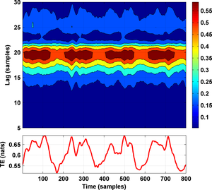
We will start by showing you what results you should obtain after a successful analysis. The transfer entropy values corresponding to the flow from the master towards the slave circuit are shown in the figure below:
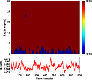
The waveform in the lower part of the figure depicts TE values at lag = 20 sampling instants. The following figure shows in dark red the pairs (lag, time instant) where the estimated TE value reached significance (p < 0.05) and in blue those where it did not reach significance:
The waveform in the lower part of the figure above depicts TE significance thresholds at lag = 20 sampling instants. Clearly, the two figures above lead us to the conclusion that the master system is exerting a major effect on the dynamics of the slave circuit, with a coupling lag of roughly 20 sampling instants. Moreover, the coupling dynamics seem to follow a strongly periodic pattern with a period of roughly 100 data samples.
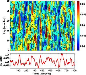
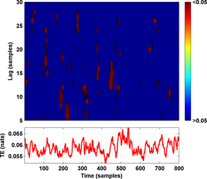
We should now repeat the steps in the previous section to assess also information flow from the slave circuit towards the master. The result would be the following two figures:
which correctly indicate that there is not any significant flow of information from slave to master at any lag.
For convenience, you can generate the four figures above by just running the following commands:
>> pset = generate_pset                       % load the dataset
>> results = tutorial_circuits_analysis(pset) % performs the TE analysis
>> tutorial_circuits_figures(results)         % generates the figures
However, the best way of learning this tutorial is that you try to re-generate
these figures without using the provided function tutorial_circuits_analysis.
Measuring information transfer
We will start our analysis by assessing information flow from the first circuit (the master) towards the second (the slave). In the following, we will refer to the master time-series as the source of the information flow and we will refer to the slave time-series as the sink of the information flow.
State-space reconstruction
Before anything else, we have to reconstruct the state-space of these scalar time-series of voltage measurements. This can be done using [delay embedding]
>> dim = 1, tau = 1;
>> Ssink = delay_embed(pset(1, :), dim, tau);
>> Ssource = delay_embed(pset(2, :), dim, tau);
where dim and tau are the embedding dimension and the embedding delay,
respectively. Choosing the right embedding parameters can be a tricky
issue. For a comprehensive review on delay embedding and state-space
reconstruction, we recommend you this book. The simplest
approach to delay embedding is to take tau = 1, dim = 1 and successively
embed in higher dimensions until the results of the analysis are consistent.
Lambda functions
For convenience, we shall define a lambda function (or function_handle
in Matlab’s terminology) as follows:
>> estimator = @(x) transfer_entropy_t(x(1,:), x(2,:), x(3,:), ...
    5, 0, 5:30, 0, 20);
This lambda function bundles together the chosen information measure
transfer_entropy_t.m with its associated input parameters
(timeWindowRadius = 5 samples, k = 20 nearest neighbors). Function
transfer_entropy_t.m requires that you specify the coupling
lag. Since this lag is unknown we entered a plausible range: 5:30.
This range will obviously vary depending on
the target application. Since we are computing the TE for 26 different lags,
the output produced by function estimator will be an array of
dimensions (26 x 1000). That is, a TE value for each lag and time instant.
Usually, time-varying estimates of information theoretic measures have a large temporal variance. If we assume that the coupling dynamics are relatively slow, we can reduce the variance by simply smoothing the estimates e.g. with a moving average filter. In order to incorporate this post-processing step, we further define the following lambda function:
>> estimator_smooth = @(x) filter(1/20*ones(1,20), 1, estimator(x), [], 2);
Temporal transfer entropy estimates
We are now ready to measure information flow from the source time-series towards the sink time-series using transfer entropy (TE):
>> W = delay_embed_future(Ssink);
>> te21 = estimator_smooth([Ssink;Ssource;W]);
where the first command builds the future of Ssink.
Assessing significance
Note: See this tutorial for a brief explanation of what significance and significance threshold mean.
Determining the significance threshold for the temporal TE estimates that we obtained in the previous section can be easily done with TIM Matlab interface using the following commands:
>> te21sig = permutation_test([Ssink; Ssource;W], [1 2 1], ...
    estimator_smooth, .05);
The last input parameter to function permutation_test.m is
the significance level or p-value. The second input parameter of function
permutation_test.m
is a vector of indices that determines how to shuffle the data trials of
each input time-series. The value [1 2 1] in the code above means that
the first (Ssink) and third (W) inputs to function
permutation_test.m should be treated as a single entity
when generating the randomly shuffled surrogates. Equivalently, this means
that, in the surrogates, the time-series Ssource will be always out-of-trial
(i.e. uncoupled) in respect to Ssink and W. See the help of
permutation_test.m and permute_pset.m
for further explanations.
Credits
German Gomez-Herrero wrote this tutorial.
The experimental measurements were obtained by Miguel C. Soriano from the Institute for Cross-Disciplinary Physics and Complex Systems, at Palma de Mallorca, Spain.


